Autonomous Shopping Robot

PythonNeural Networks

Jul 2024 - Oct 2024

A fully autonomous robot capable of collecting items on a shopping list through heavy use of computer vision, SLAM and path planning.

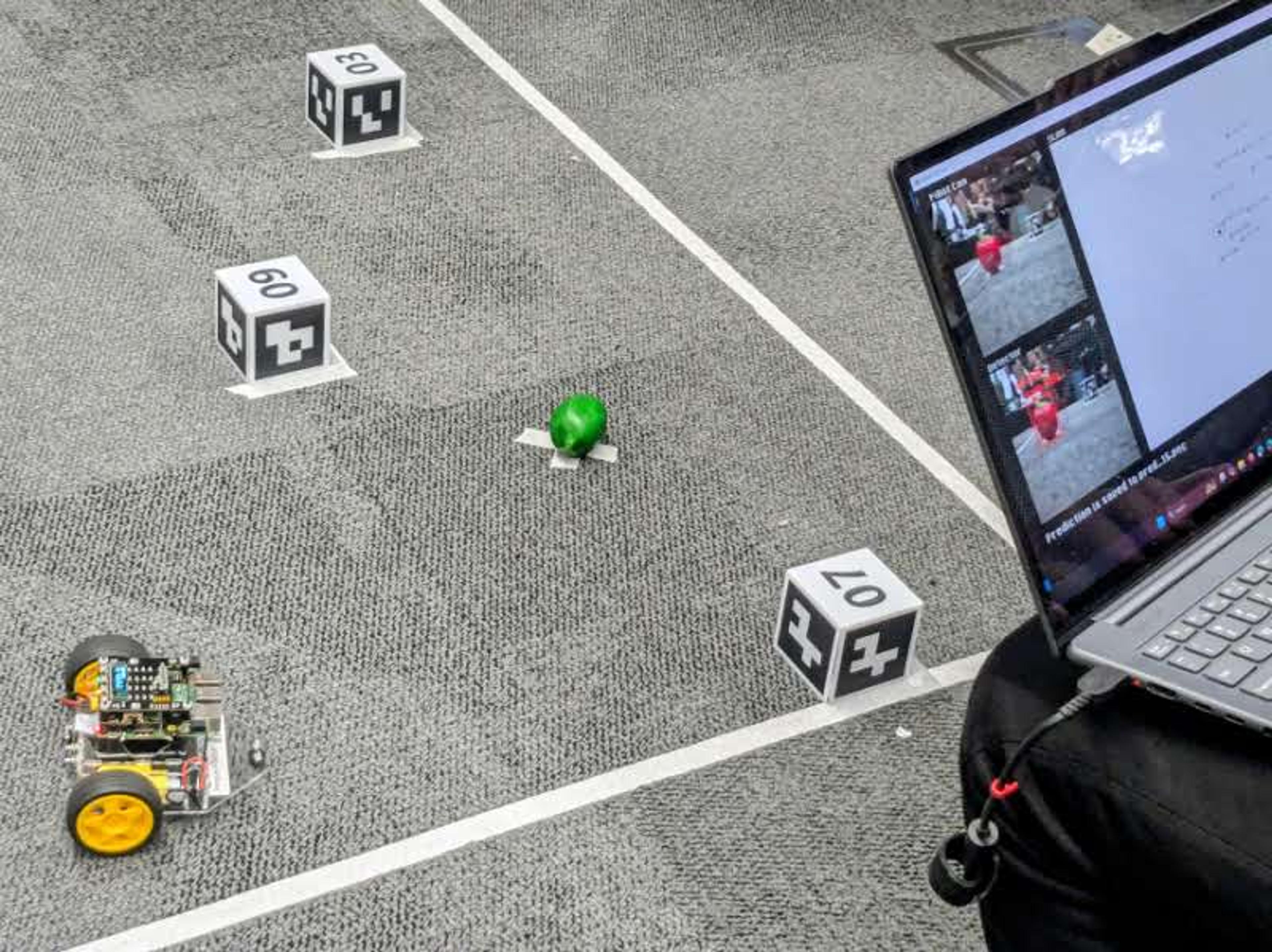
The Autonomous Shopping Robot was made with a simple goal. Given a shopping list, find and collect all the items in the shortest amount of time without crashing into the supermarket environment. The list is random, the supermarket layout changes every time and the robot goes into the challenge with no human intervention. What follows is a lot of interesting maths, computer vision techniques and machine learning to navigate and identify fruits and vegetables in the supermarket.

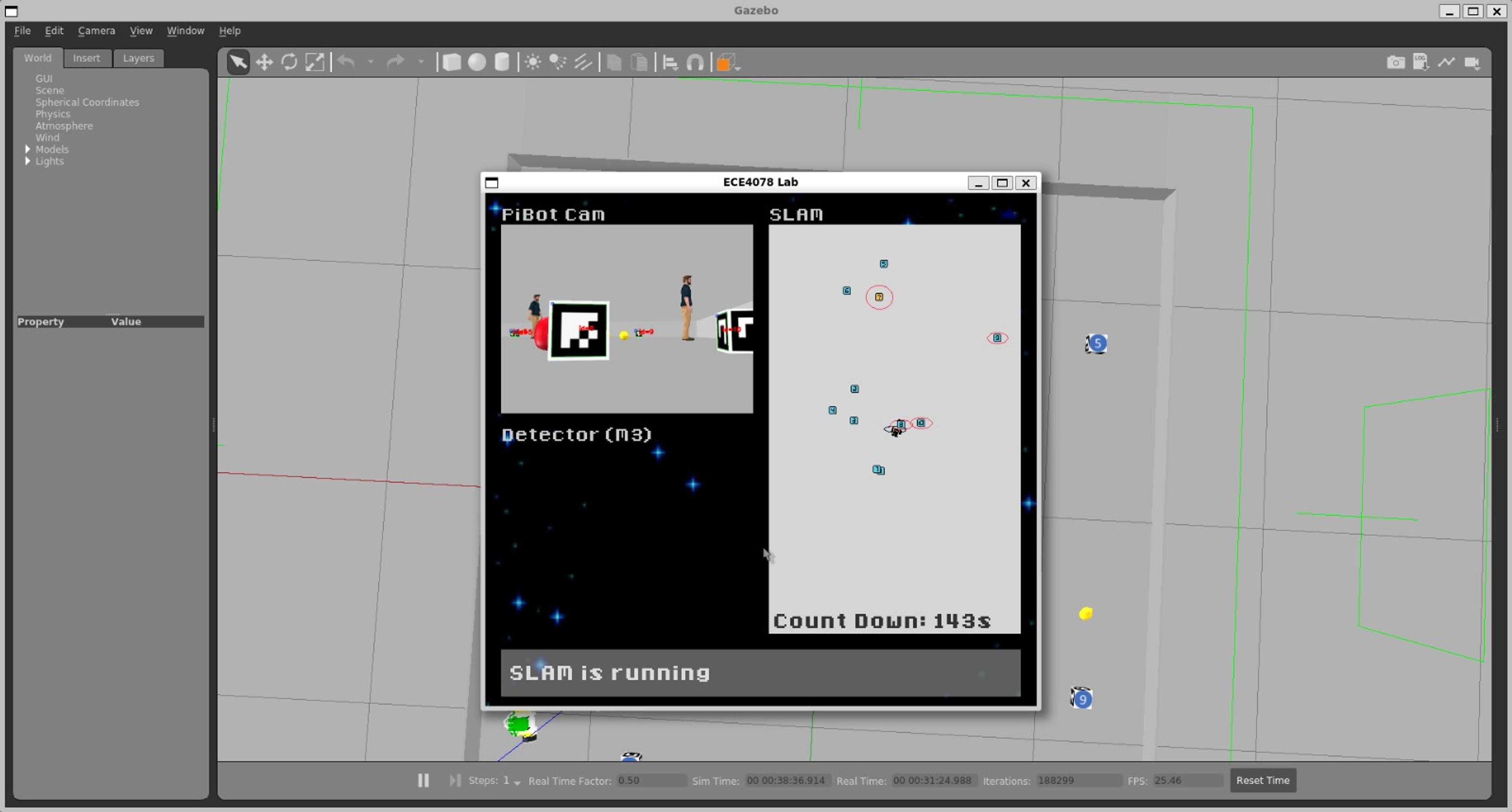
Simultaneous Localisation & Mapping (SLAM)

SLAM is the process of positioning yourself in the world while also mapping the world around you with a global source of truth. A combination of a physics model (predicting where the robot should be given a duty cycle applied to its motors over time) and sensors provide the information used to estimate where the robot is relative to the objects around it. In this environment, the ARUCO markers and the target produce act as waypoints, although their pose and position needs to be determined at runtime. It's important to note that this robot is relatively simple. The only inputs it takes are left and right wheel velocities, and the only data it returns is the current camera view.

The robot simulation environment. — The physics of the real world is simulated to assist in rapidly testing and improving the SLAM algorithms. The image shows the simulated environment and the background and the robots vision, along with ARUCO detections and the generated map. Note the covariance rings surrounding the robot and the sighted markers.

The state of our system is simply the position and rotation of the robot $x, y, \theta$ and the positions of each marker, $\mathbf{m}_i$ . This represents all the information that we want to collect about the world through measurements and motion model predictions.

\mathbf{x} = \begin{bmatrix} x \\ y \\ \theta \\ \mathbf{m}_1 \\ \mathbf{m}_2 \\ \vdots \\ \mathbf{m}_N \end{bmatrix}, \qquad \mathbf{m}_i = \begin{bmatrix} x_i \\ y_i \end{bmatrix}

Modelling Motion

As previously mentioned, there are two parts to SLAM; the motion model and the measurements. We can ignore the ARUCO markers for this part as they haven't grown legs yet. On the other hand, the robot can move. Given that the robot only has two wheels, the equations giving the motion model are quite simple. If the wheels are being driven at the same speed, we can assume linear motion with acceleration being negligible as the motors are electric and the period of acceleration is minimal compared to the time driven at speed. This effectively means that we can simply multiply the linear velocity by the time travelled to find the distance travelled. Mapping the linear velocity to the motor duty cycles is simply a matter of finding calibration constants (constants not constant as friction is a non-linear force) for difference linear velocities.

v=\frac{c(l+r)}{2}\\\\ \omega=\frac{c(r-l)}{b}

Where $c$ is the scaling factor and $b$ is the base width, the distance between the two wheels. Knowing the previous state $\textbf{x}_{k-1}$ , the control inputs $\mathbf{u}_k= \begin{bmatrix} v_k & \omega_k \end{bmatrix}'$ and the time since the last measurement $\delta t$ , we can model the motion of the robot.

When $\omega=0$ :

\mathbf{f}(\mathbf{x}_{k-1}, \mathbf{u}_{k-1})= \begin{bmatrix} x_{k} \\ y_{k} \\ \theta_{k} \end{bmatrix} = \begin{bmatrix} x_{k-1} + v_k \cos(\theta_{k-1})\, \delta t \\ y_{k-1} + v_k \sin(\theta_{k-1})\, \delta t \\ \theta_{k-1} \end{bmatrix}

When $\omega \neq 0$ :

\mathbf{f}(\mathbf{x}_{k-1}, \mathbf{u}_{k})= \begin{bmatrix} x_{k} \\ y_{k} \\ \theta_{k} \end{bmatrix} = \begin{bmatrix} x_{k-1} + \frac{v_k}{\omega_k}\left(\sin(\theta_{k-1} + \omega_k \delta t) - \sin(\theta_{k-1})\right) \\ y_{k-1} - \frac{v_k}{\omega_k}\left(\cos(\theta_{k-1} + \omega_k \delta t) - \cos(\theta_{k-1})\right) \\ \theta_{k-1} + \omega_k \delta t \end{bmatrix}

These equations give a complete picture as to how the robot moves, in response to control signals given to the wheels. As each movement carries some uncertainty as our motion model doesn't account for every last physical interaction, we describe our state with a probability distribution. This distribution is modelled as normal distribution about $\textbf{0}$ with a configurable variance $\textbf{Q}$ .

\mathbf{x}_k = \mathbf{f}(\mathbf{x}_{k-1}, \mathbf{u}_k) + \mathcal{N}(\mathbf{0}, \mathbf{Q})

In practice we store and calculate the means and covariance separately, however the two combined fundamentally form the complete state.

Taking Measurements

One we've taken a measurement and found the visible markers positions in the world frame, we need to convert them to the robot frame using the current robot state:

R(\theta) = \begin{bmatrix} \cos\theta & -\sin\theta \\ \sin\theta & \cos\theta \end{bmatrix} \\\mathbf{z}^{\mathrm{r}}_i = R(\theta)^\top \left( \mathbf{p}^w_i - \begin{bmatrix} x \\ y \end{bmatrix} \right)

Kalman Filters

The power of the Kalman filter occurs when we combine the motion model with the measurements to produce a better estimate than either one of these values alone. However, Kalman filters require a linear model, while our motion and measurement models are non-linear. This is not a problem as we can locally linearise each model at every time step $k$ to provide a close-enough approximation. This done by taking the first order Taylor series expansion (though high orders are possible too, but often not necessary). For this we simply need the first derivative at the previous state $\textbf{x}_{k-1}$ .

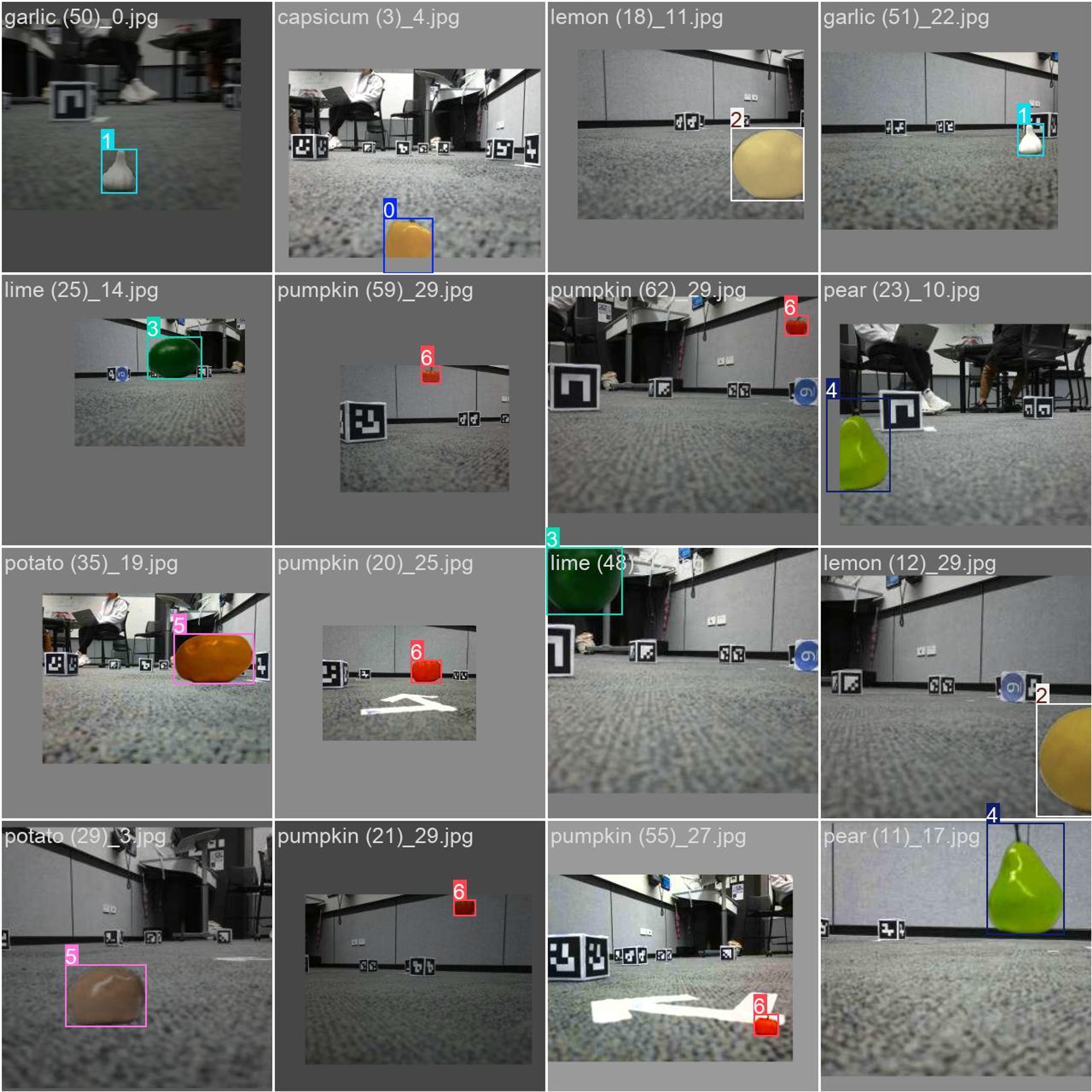
Target Detection

The identification of targets (i.e. fruits and vegetables) is completed through the industry standard object recognition and segmentation model, YOLOv8. The model was trained on 10,000 images of the fresh produce on a variety of backgrounds, however these images weren't manually labelled as this would be incredibly time consuming. Instead, a custom dataset generator was built to superimpose the fresh produce on a variety of backgrounds, while applying a variety of augmentations to improve the robustness of detections.

A variety of detections on the generated test dataset.

Approximately 100 photos of the fresh produce were taken from the robot camera against a plain white background. Only the angle of the targets relative to the robot was varied in between shots.
The backgrounds were automatically removed using a simple Python script, resulting in hundreds of labelled produce images with a transparent background.
Various background photos were taken, ensuring that none of the images included the target. The produce images were superimposed onto these backgrounds, resulting image that resembled the authentic environment, except that the class and bounding box can be automatically assigned. While the images were superimposed, various augmentations were randomly applied, such as:
- Brightness
- Rotation
- Flipping
- Scaling
- Translation
- Blurring
- Hue-shifting

Once trained on these generated images, the model was incredibly reliable with >99% recall on an unseen test dataset and strong realtime performance in the trial environments.

Clustering & Pose Estimation

As explored earlier in the section on SLAM, we map out the produce as the robot drives around by combining estimates of the robots position and measurements taken from the camera feed. However, the next question that follows is how do we measure the relative position of the produce? Assuming fixed size produce, we can use similar triangles and the intrinsic matrix to find the distance and angle relative to the robot. This measurement can then be projected from the robot frame to the world frame to provide a position estimate for our produce.

Over time, we gather hundreds of unique estimates as to where a class of produce is, but this doesn't mean that there are equally many instances of this item in the real world. In fact, we may only have 1 or 2 pieces of garlic in a given space, but 300 slightly different position estimates. To resolve this, we employ DBSCAN clustering to group these estimates into a handful of usable positions.