Neural Cellular Automata

Nov 2024 - Nov 2025

Using Neural Networks to simulate life with cellular automata.

The Neural Cellular Automata project is a research project under Monash DeepNeuron; an AI and HPC student team at Monash University. Neural Cellular Automata is an emerging research field, enabled by recent improvements in compute that combines the powers of localised behaviour with the learnable parameters of neural networks.

Cellular Automata

Before understanding Neural Cellular Automata (NCA), it's only natural to cover Cellular Automata (CA), the superset of NCA first. Cellular Automata are cells (which may be pixels, voxels or a vertex on any graph), each of which has a state. In classical CA, like the famous Conway's Game of Life, this state is a binary on/off. From each cell's state, and the state of its immediate neighbours, the next state can be computed using a single rule.

• Decentralised Control: each cell "thinks" for itself, in the way that the update rule is only provided with the state of the current cell and its neighbours, there is no central control instructing how each cell should change.
• Emergent Behaviour: from simple rules and local interactions emerges growth, movement and pattern-formation.
• Parallelisable Computation: as each cell is effectively independent from each other, the next state computations of CAs are highly parallelisable, lending themselves naturally to the GPU.

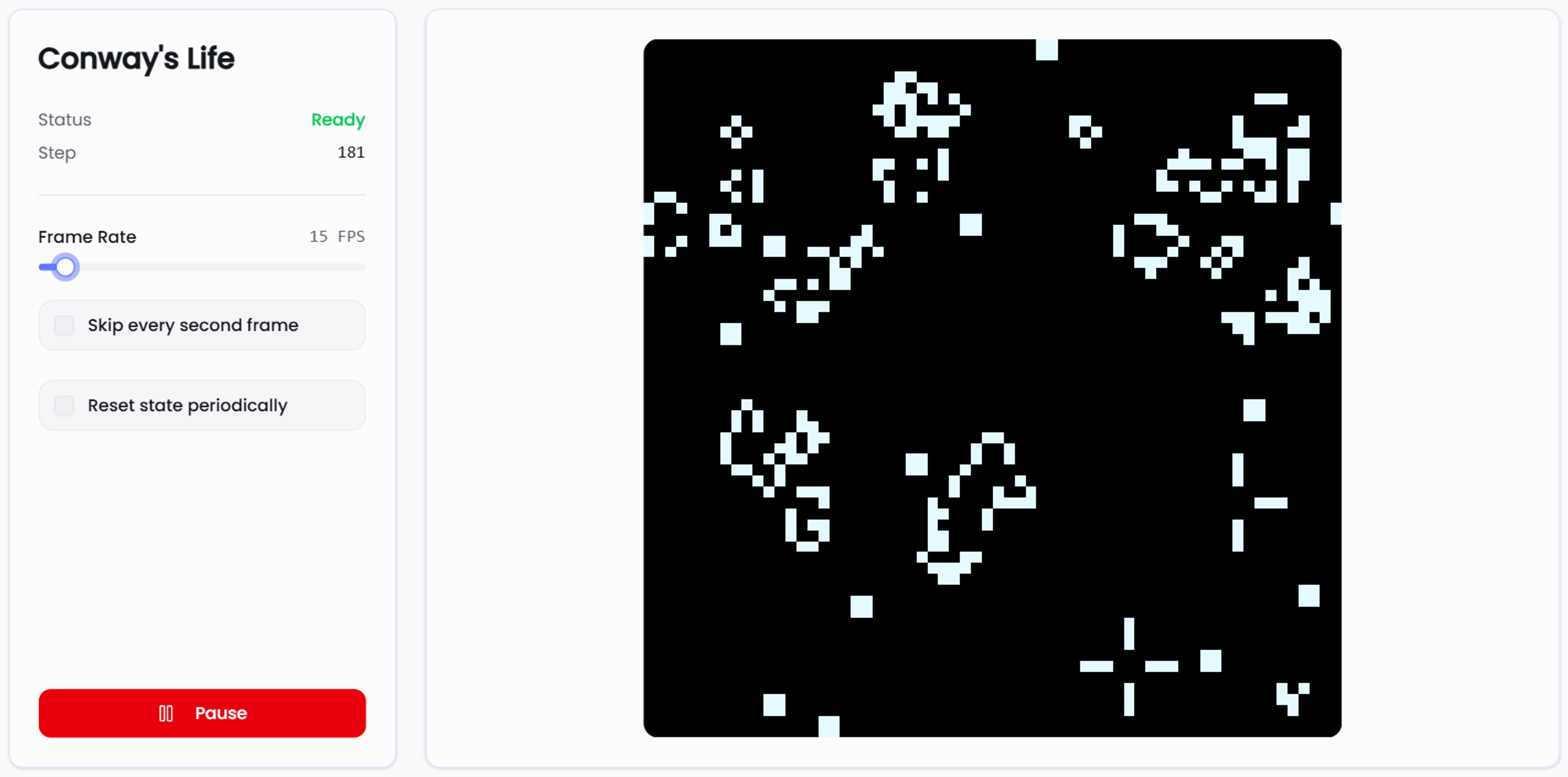
John Conway's Game of Life

John Conway's Game of Life is one of the simplest CA rulesets that still yields very interesting behaviour. The game takes place on a 2D grid, where each cell is a dead (black) or alive (white). The ruleset is as follows:

• Each cell with one or fewer alive neighbours will die next turn.
• A cell with 2 or 3 alive neighbours will live.
• Cells with 4 or more alive neighbours will die as if by overcrowding.

From these rules common patterns such as blocks, blinkers and spaceships emerge. Check out our simulation on the NeuralCA website to see them for yourself.

Continuous Cellular Automata

While classical models such as Conway's Life and Larger than Life employ a simple binary state, there's no reason why we can't swap our state for continuous values from 0 to 1 and our ruleset with equations. This is the next logical step towards NCA. By instead using the single value as a measure of brightness, our life becomes a touch more complex.

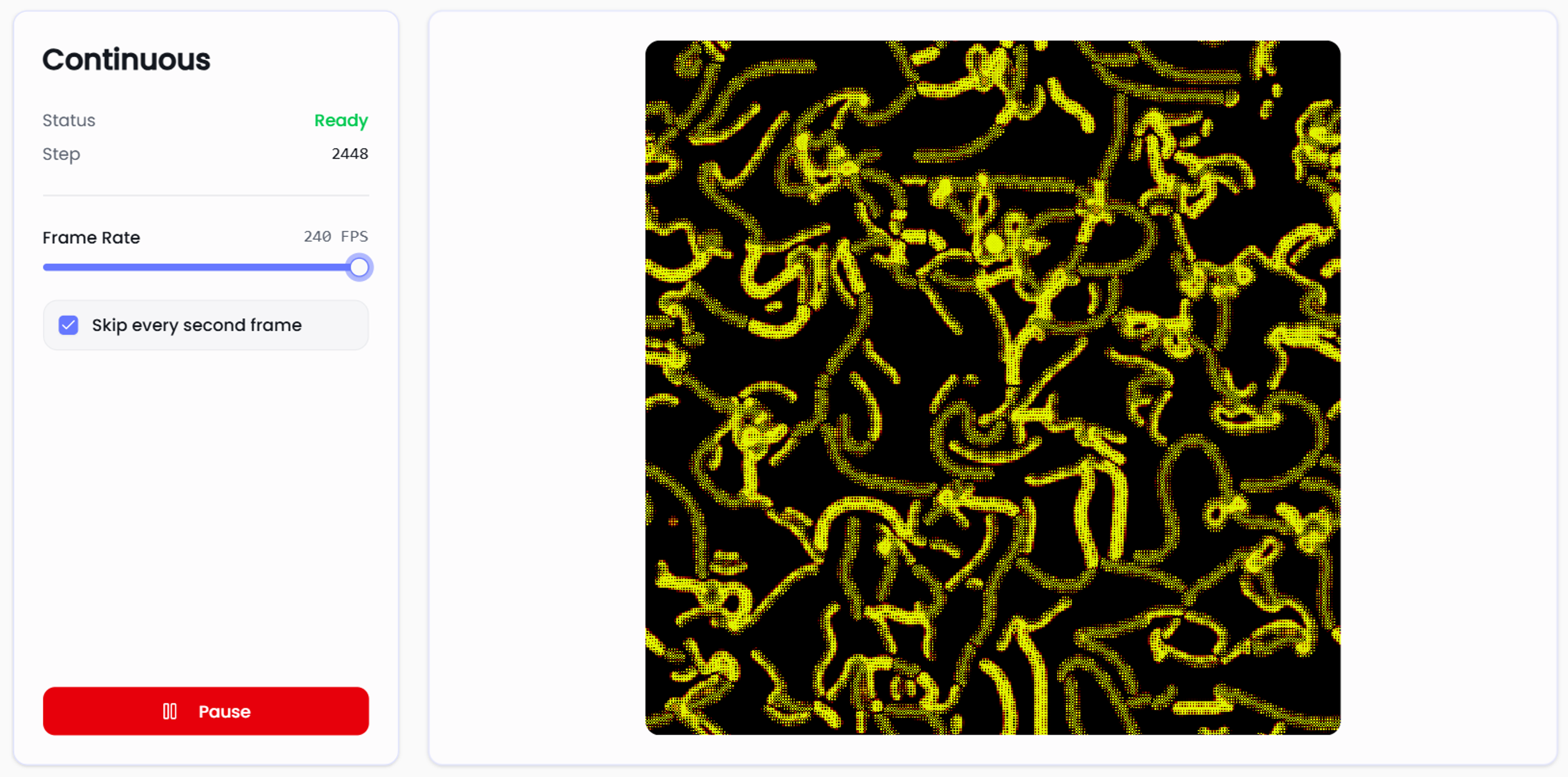
A continous state increases the amount of information stored in each cell, allowing for complex patterns and form to emerge.

Neural Cellular Automata

Until now, the next state has been a product of the current state and the cell's 8 immediate neighbours. With Neural Cellular Automata... this doesn't change. Instead of defining a ruleset based on a series of logical conditions or a mathematical formula, instead we drop in a neural network with learned parameters. Just like how our DNA has evolved over time, the training of NCA is not too dissimilar. We first initialise our parameters with random values, let the cells run in a while and we then update the weights to more closely resemble behaviour we want to see. One of the most influential papers in this field came in 2020, titles Growing Neural Cellular Automata as it laid out some of the fundamentals of NCA.

• Differentiable: the update rule needs to be differentiable from start to finish in order to be able to backpropagate losses.
• Simple Architectures: given each cell on the grid has to run a forward pass for every update step, if we want to achieve a smooth frame rate with an acceptable resolution, we need to keep the networks small. For NCA, only 2 or 3 fully-connected layers are required with very few parameters.

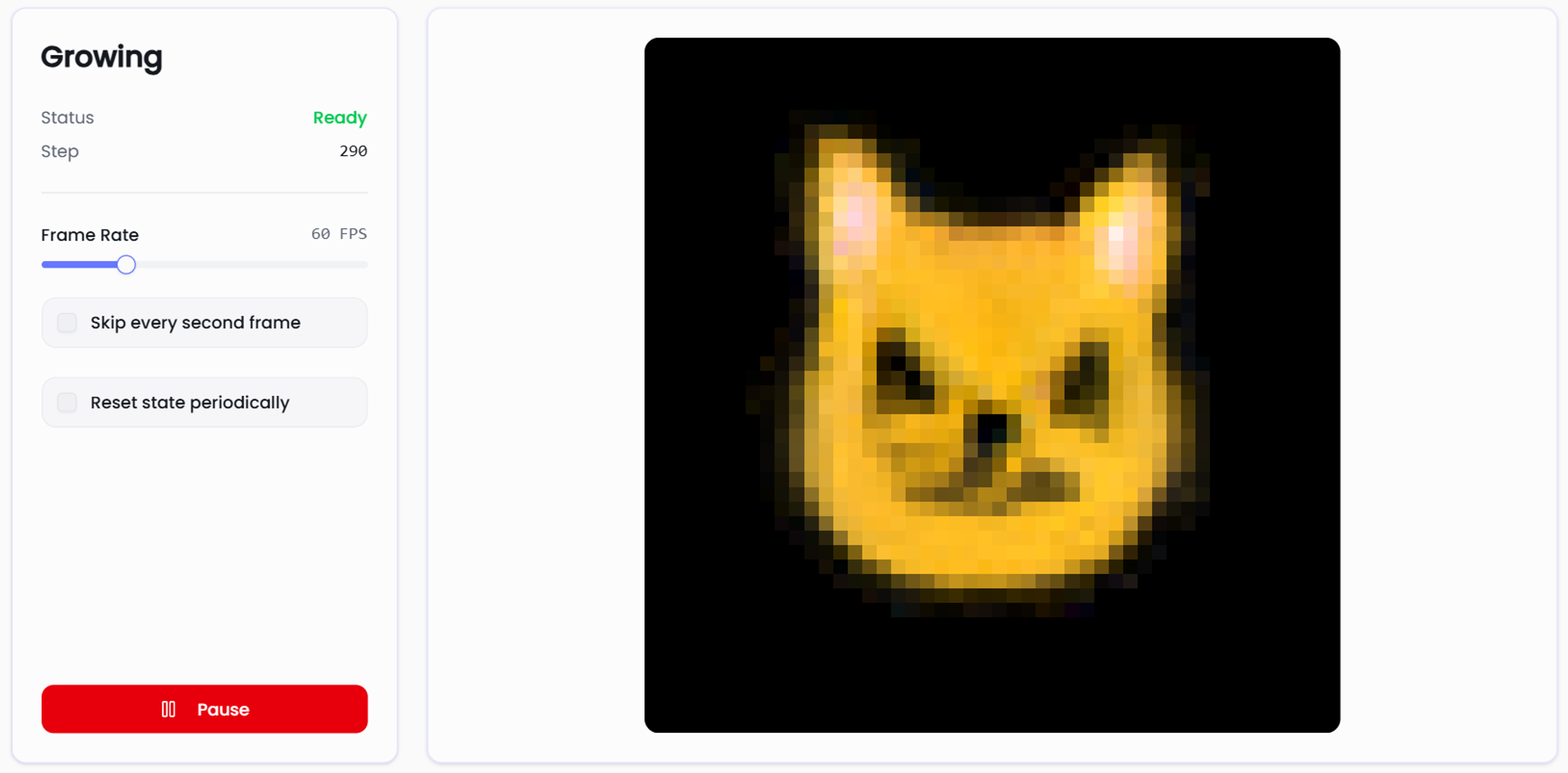
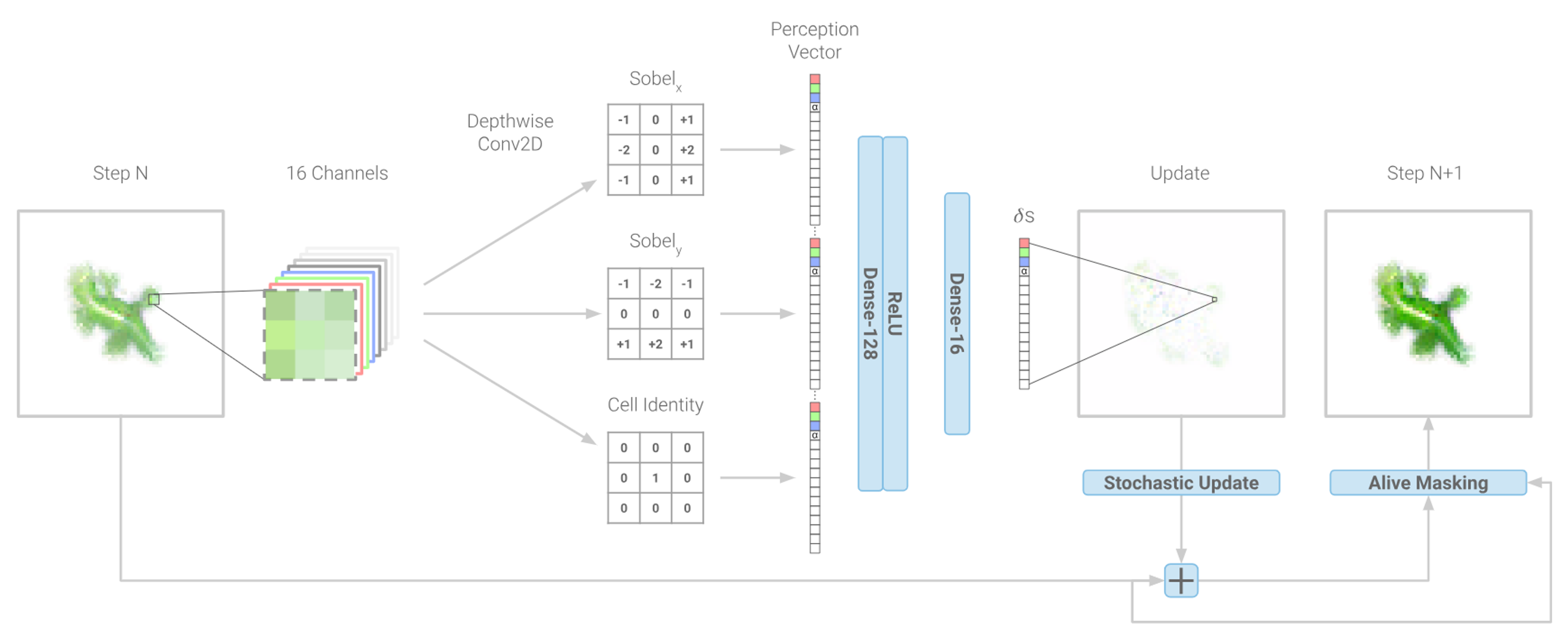
It's worth noting that the state is a bit more complex here. While before we say a single floating point value represent the entire state of a cell, with NCA we expand this state to a vector of floating point values. The Growing model has 16 channels:

• 3 Visible Channels, denoting red, green and blue respectively.
• 1 Alpha Channel determining whether the cell should be considered dead or alive.
• 12 Hidden Channels that the network can decide to use however it likes to convey information to its neighbours.

Training NCA

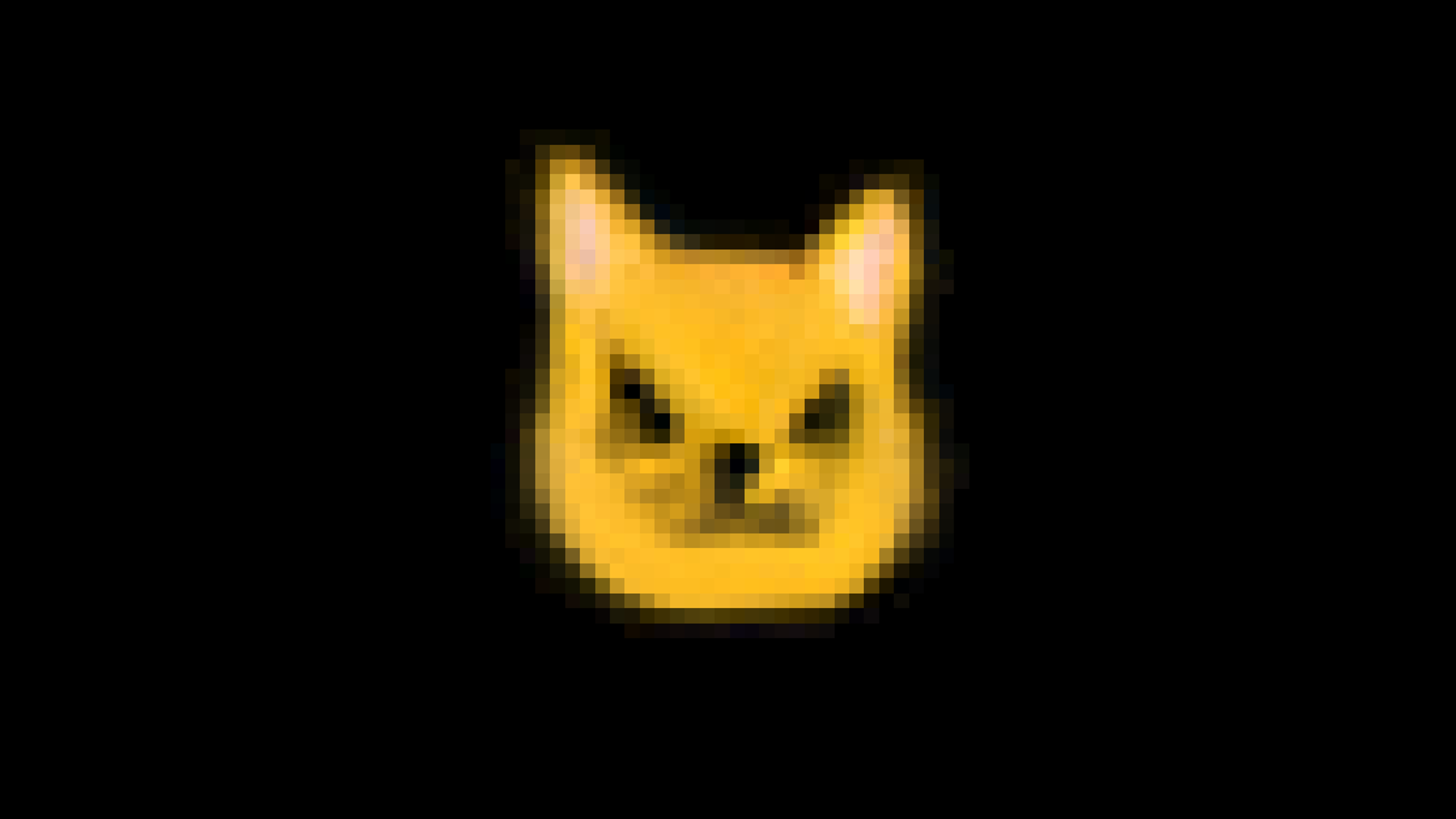
Given the architecture of NCA is so simple, much of the complexity lies in the loss function used to train it. While the Growing model uses a single target image and computes a loss based on the sum of squared differences (SSD) between the current CA state and the target, we can go further and implement less obvious loss functions. A prime example of this is the Texture model that seeks to emulate the look and feel of an image, rather than replicating the target exactly. What results is an image that is not temporally stable, but uses the same colours, shapes and arrangement as was seen in the target.

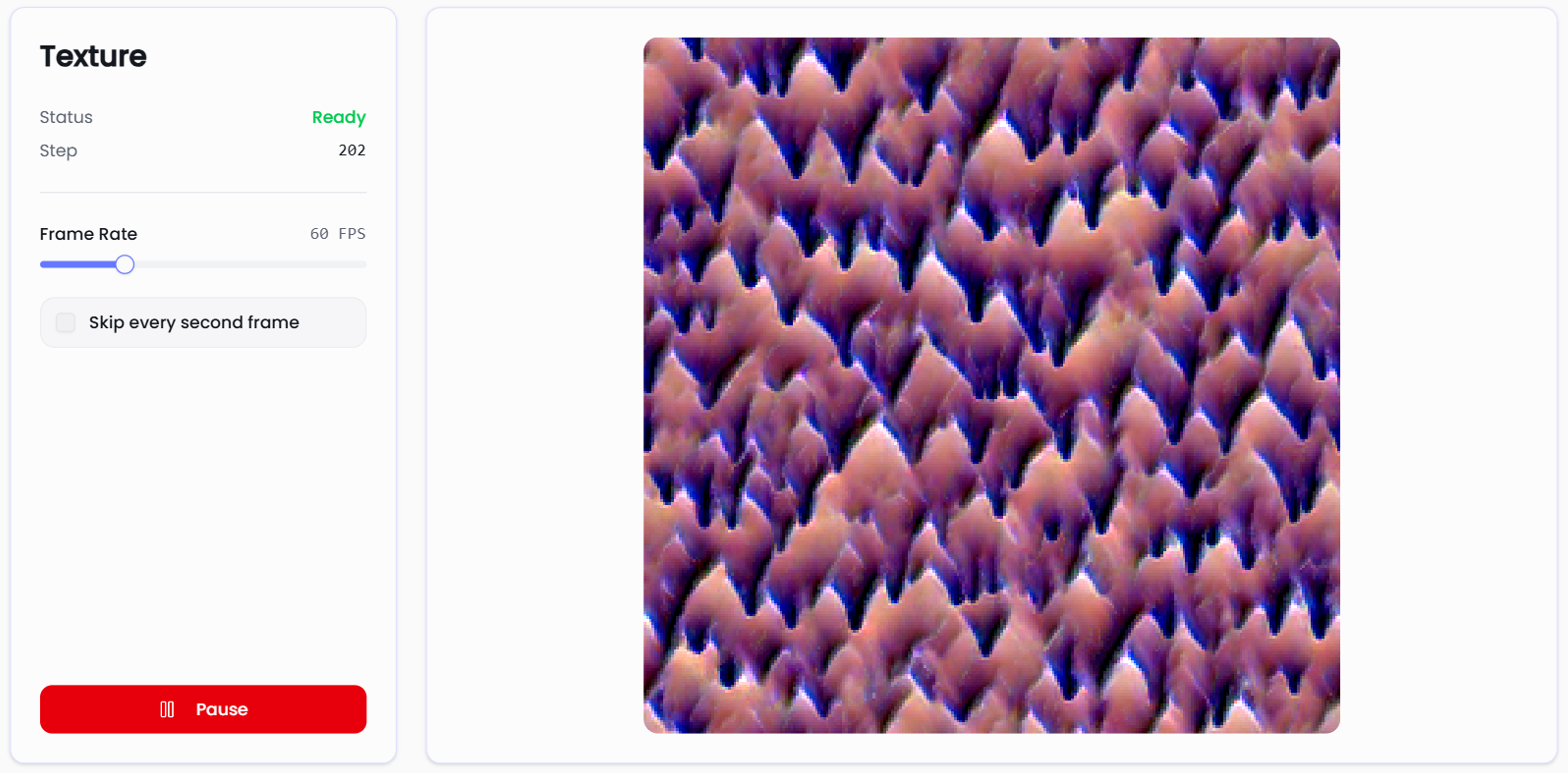
A great way to programmatically define "the feel" of images is to use the feature layers of image recognition networks such as VGG-16. Fundamentally, image recognition networks use colours, shapes and patterns in order to recognise objects or in this case, classify textures. Thus, if we compare the features that are activated when we pass our target image through VGG-16 to the features activated when we pass our NCA through, what we find a difference, or in other words, a loss.

Live Client-Side Demos

Unfortunately, the applications of NCA beyond biology modelling and texture generation are quite limited, but that doesn't stop them from being beautiful and fascinating. In this spirit, and as referenced throughout this page already, the Neural Cellular Automata team at Monash DeepNeuron has gone about re-implementing all these models in WebGPU Shader Language so they can be performantly run on a client device in real-time.

The WebGPU API is the successor to the WebGL API, offering access to the device's GPU hardware to run render and compute shaders. This project makes use of these render shaders to draw the final result, but more importantly the compute shaders to run the millions of convolutions and neural network forward passes each second.

Every detail of these shaders was optimised to squeeze out as many frames as possible from lower end devices. Take for example the 2D convolution function, which needs to perform the spatial convolution with circular padding.

1// Helper function to perform convolution with a 3x3 kernel for a specific channel
2fn convolve(c: u32, x: u32, y: u32, kernel: mat3x3f) -> f32 {
3  let size = shape.size;
4  var sum: f32 = 0.0;
5
6  for (var ky = 0u; ky < 3u; ky++) {
7    for (var kx = 0u; kx < 3u; kx++) {
8      // Find neighbours with circular padding
9      let dx = (x + kx - 1 + size) % size;
10      let dy = (y + ky - 1 + size) % size;
11      let i = index(c, dx, dy);
12      sum += state[i] * kernel[ky][kx];
13    }
14  }
15
16  return sum;
17}

To prevent casting from signed integer indexes i32 back to unsigned integers u32, the indices are instead left as unsigned integers. First, the offset kx or ky (ranging from 0 to 2) is added then scaled back to the correct range (-1 to 1). This step could be further reduced to 2 operations if we instead use integer overflow to accomplish this task, however this technique obscures the intention from the compiler, potentially stripping away automatic loop unrolling from certain implementations. We then add the size of the image grid, size, to the result, accounting for the case where we wrap around with negative indices. Finally, we take the modulo size to account for the case where the wrap around to the right of the grid.

It may seem more intuitive to perform these operations with simple if statements, but there is a reason that we go to great length to avoid them. Branching, especially in hot loops like this one (which will run millions of times a second) is incredibly slow as it causes per pixel divergence. This same concept applies to stochastic masking, it is faster to apply a random mask to an already computed result than it is to conditionally skip it on a per pixel basis.